How to draw OpenCV Mat data into native Windows client area utilizing GDI

under some scenario, probably one wants to combine the OpenCV's ability to manipulate pixel values, and the Windows ability to display the resulting image in a native way (for example, utilizing the GDI system). Such a requirement demands some deep understanding of image representation between these two systems, and probably a non-trivial task than just taking for granted.


I came across a same situation as just mentioned above, and after some try-and-error iteration, finally everything seems have been put onto track. since it hasn't undergone thorough test, I am not sure the tracks are all right tracks.

would like to share here for polishing or beneficial for others facing the same situation.

The header file is as follows:

#pragma once

#include <opencv2/core.hpp>

class COpenCVImage
{
public:
COpenCVImage(LPCTSTR lpszFileName);
~COpenCVImage(void);

BOOL GetSize(LPRECT lpRect);
BOOL DrawBitmap(HDC hdc, LPRECT lpRect);

BOOL Sharpen(HWND hWnd);
BOOL Flip(HWND hWnd);

private:
bool createBitmap(HDC hdc, cv::Mat mat);
private:
cv::Mat m_matImage;
HBITMAP m_hBitmap;

bool m_bInit;
};


the implementation file is as follows:

#include "stdafx.h"
#include "OpenCVImage.h"

#include <Shlwapi.h>
// The following header file will be excluded, since we will draw the picture 
// to the window all by ourselves
// #include <opencv2/highgui.hpp>
#include <opencv2/imgcodecs.hpp>
#include <opencv2/imgproc.hpp>

COpenCVImage::COpenCVImage(LPCTSTR lpszFileName) : m_hBitmap(NULL), m_bInit(false)
{
if(!PathFileExists(lpszFileName))
{
MessageBox(NULL, _T("Cannot open the image file"), _T("Error"), MB_OK);
return ;
}

char* pFileName;
UINT nLen;

nLen = WideCharToMultiByte(CP_UTF8, 0, lpszFileName, sizeof(TCHAR) * (_tcslen(lpszFileName) + 1), NULL, 0, NULL, NULL);
pFileName = new char[nLen];
WideCharToMultiByte(CP_UTF8, 0, lpszFileName, sizeof(TCHAR) * (_tcslen(lpszFileName) + 1), pFileName, nLen, NULL, NULL);

m_matImage = cv::imread(pFileName, cv::IMREAD_COLOR);
delete [] pFileName;

if (m_matImage.empty())
{
MessageBox(NULL, _T("Cannot read in the image file"), _T("Error"), MB_OK);
return;
}

m_bInit = true;
}

COpenCVImage::~COpenCVImage(void)
{
if (m_hBitmap)
DeleteObject(m_hBitmap);
}


BOOL COpenCVImage::DrawBitmap(HDC hdc, LPRECT lpRect)
{
if (!m_bInit)
return FALSE;

HDC hDCMem = CreateCompatibleDC(hdc);

if (!m_hBitmap)
{
createBitmap(hDCMem, m_matImage);
}

SelectObject(hDCMem, m_hBitmap);

BitBlt(hdc, lpRect->left, lpRect->top, lpRect->right - lpRect->left, 
lpRect->bottom - lpRect->top, hDCMem, 0, 0, SRCCOPY);

DeleteDC(hDCMem);

return TRUE;
}


BOOL COpenCVImage::GetSize(LPRECT lpRect)
{
if (!m_bInit)
{
memset(lpRect, 0, sizeof(RECT));
return FALSE;
}

lpRect->left = 0;
lpRect->top = 0;
lpRect->right = m_matImage.cols;
lpRect->bottom = m_matImage.rows;

return TRUE;
}

BOOL COpenCVImage::Sharpen(HWND hWnd)
{
if (!m_bInit)
return FALSE;

cv::Mat matFiltImage;
cv::Matx33f matKernel;

matKernel(1, 1) = 5.0;
matKernel(0, 1) = - 1.0;
matKernel(1, 0) = - 1.0;
matKernel(1, 2) = - 1.0;
matKernel(2, 1) = - 1.0;

cv::filter2D(m_matImage, matFiltImage, m_matImage.depth(), matKernel);

HDC hDCMem = CreateCompatibleDC(GetDC(hWnd));
createBitmap(hDCMem, matFiltImage);
DeleteObject(hDCMem);

InvalidateRect(hWnd, NULL, TRUE);

return TRUE;
}

BOOL COpenCVImage::Flip(HWND hWnd)
{
if (!m_bInit)
return FALSE;

cv::Mat matFlipImage;
cv::flip(m_matImage, matFlipImage, 1);

HDC hDCMem = CreateCompatibleDC(GetDC(hWnd));
createBitmap(hDCMem, matFlipImage);
DeleteObject(hDCMem);

InvalidateRect(hWnd, NULL, TRUE);

return TRUE;
}

bool COpenCVImage::createBitmap(HDC hdc, cv::Mat mat)
{
unsigned char* lpBitmapBits;

if (m_hBitmap)
DeleteObject(m_hBitmap);

BITMAPINFO bi; 
ZeroMemory(&bi, sizeof(BITMAPINFO));
bi.bmiHeader.biSize = sizeof(BITMAPINFOHEADER);
bi.bmiHeader.biWidth = m_matImage.cols;
bi.bmiHeader.biHeight = - m_matImage.rows;
bi.bmiHeader.biPlanes = 1;
bi.bmiHeader.biBitCount = (m_matImage.elemSize() << 3);
bi.bmiHeader.biCompression = BI_RGB;

m_hBitmap = CreateDIBSection(hdc, &bi, DIB_RGB_COLORS, (VOID**)&lpBitmapBits, NULL, 0);

#define ALIGN(x,a)              __ALIGN_MASK(x, a-1)
#define __ALIGN_MASK(x,mask)    (((x)+(mask))&~(mask))
int width = m_matImage.cols * m_matImage.elemSize();
int pitch = ALIGN(width, 4);
#undef __ALIGN_MASK
#undef ALIGN

for(int i = 0; i < m_matImage.rows; i ++)
{
unsigned char* data = mat.ptr<unsigned char>(i);
memcpy(lpBitmapBits, data, width);
lpBitmapBits += pitch;
}

return true;
}

a typical usage probably be:

1. instantiate the instance, for example:
COpenCVImage image(_T("lenna.jpg"));

2. respond to the WM_PAINT message:

case WM_PAINT:
hdc = BeginPaint(hWnd, &ps);
// TODO: Add any drawing code here...

RECT rect;
image.GetSize(&rect);
image.DrawBitmap(hdc, &rect);

EndPaint(hWnd, &ps);

break;


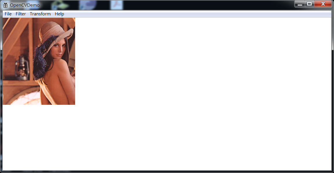
the final result is as follows:

appreciate any suggestion to enhance the code

Fourier in image processing (I)

before indulge into the frequency field of image processing, two points must be manifested:

1. the mathematical rigor is a good thing, however in practice just stick to it in some extent in case of seeking trouble for oneself. so don't be panic if you see someone exchange summation and integration freely.

2. casualness doesn't give one enough reason to neglect some basic concepts concerning with Fourier theory, like the difference between Fourier series and Fourier transform. otherwise, your further deduction probably in the wrong track.

fft: fast Fourier transform for 1-D vector
Note, to really utilize the virtue of fft, the size of vector must a power of 2. otherwise it will fall back to the general discrete Fourier transform
example:
u = [1, 2, 4, 1];
F = fft(u);

the result is as follows:
F = [8.0000 + 0.0000i  -3.0000 - 1.0000i   2.0000 + 0.0000i  -3.0000 + 1.0000i]

fft2: fast Fourier transform for 2-D matrix
identical to fft, if the size of matrix along some dimension is not the power of 2, along that dimension, it automatically falls back into discrete Fourier transform.
example:
S = fspecial('sobel');
F = fft2(S);

the results are as follows:
S = [

     1     2     1
     0     0     0
    -1    -2    -1
];
F = [
   0.0000 + 0.0000i   0.0000 + 0.0000i   0.0000 + 0.0000i
   6.0000 - 3.4641i  -1.5000 - 0.8660i  -0.0000 + 1.7321i
   6.0000 + 3.4641i  -0.0000 - 1.7321i  -1.5000 + 0.8660i
];

fftshift: shift the DC component to the center in order to benefit inspection

example:
FC = fftshift(F);

the result is as follows:
FC = [

  -1.5000 + 0.8660i   6.0000 + 3.4641i  -0.0000 - 1.7321i
   0.0000 + 0.0000i   0.0000 + 0.0000i   0.0000 + 0.0000i
  -0.0000 + 1.7321i   6.0000 - 3.4641i  -1.5000 - 0.8660i
];

ifftshift: inverse of fftshift

following, i will give a comprehensive example to demonstrate the usage of above functions. the purpose of the example is apply low-pass filter in the frequency domain to some image, so as to observe the results:

function freqfilt(img_path)

try
    img = imread(img_path);
catch
    msgbox('cannot open image file, check the file name!');
    return ;
end

h1 = figure(1); imshow(img);
figure(h1); title('Original image');

% Convert into gray-level image if necessary. you've been warned

% FFT transform
img_freq = fft2(img);

% Shift the DC component into center for observing
img_freq = fftshift(img_freq);

% Adjust the frequency value for displaying
img_freq_mag = abs(img_freq);
img_freq_mod = log(img_freq_mag + 1);

% Normalize the matrix since elements are of floating point datatype

f_max = max(max(img_freq_mod));
img_freq_mod = img_freq_mod / f_max;

h2 = figure(2); imshow(img_freq_mod);
figure(h2); title('Spectrum distribution');

% Create a mask for frequency filed filting
[cx, cy] = size(img);

mask = bsxfun(@plus, ((1:cx) - ceil(cx/2)) .^ 2, (transpose(1:cy) - ceil(cy/2)) .^ 2) < 100^2;
h3 = figure(3); imshow(uint8(mask * 255));
figure(h3); title('Mask image');

% Do the filting
img_freq = img_freq .* mask;

% Shift the freqency back to do inverse fft
img_freq = ifftshift(img_freq);

% Note the relation between ifft by utilizing forwarding fft
img_freq = img_freq';
img_ift = fft2(img_freq);
img_ift = img_ift' / numel(img);

% Trucate to real numbers to surpress round-off error
img_ift = real(img_ift);

h4 = figure(4); imshow(uint8(img_ift));
figure(h4); title('Filtered image');

the results are as follows:

imfilter: filtering a given image with specific kernel
example:
img = imfilter(rgb2gray(imread('test.jpg')), fspecial('guassian'));

note, for all kinds of filters, a normalization is recommended before applying to the image. for low pass filter, it's not necessary for adding the original image for displaying. generally for high pass filter, it's tended to request adding the original image before displaying.

freqz2: frequency response for 2-D matrices.
note, this function is mainly for testing kernels, architect your own utility to display the spectrum of some large image.
example:
freqz2(fspecial('laplacian'));

the result is as follows:

Matlab functions and image processing toolbox functions summary (I)

imread: load an image into matlab workspace

imshow: show an loaded image or synthetic image by some special matrix

example:
img_color = imread('forest.jpeg', 'jpg');
imshow(img_color);

the figure being shown is as follows:

rgb2gray: convert a color image to an gray-level image

example: 
img_gray = rgb2gray(img_color);


imhist: demonstrate the histogram of an image. note this routine can only apply to gray-level image. the answer is color image is generally abundant with intensity values, (255x255x255), such a sparse intensity over weight demonstration is of little meaningfulness.

example:
imhist(img_gray);

the result is as follows:

histeq: do the histogram equalization to specific image

example:
img_eq = histeq(img_gray);
imshow(img_eq);

the result is as follows:

graythresh: compute the threshold for a given image
im2bw: convert an image into black-white image

note above the above function are tended to use jointly
gt = graythresh(img_gray);
img_bw = im2bw(img_gray, gt);
imshow(img_bw);

the result is as follows:

note the above example is operated upon image with data type unsigned char. however it could also be operated on float number. refer to the following example, but before that, let's introduce another function:
im2double: convert the intensity value into double float number

so the final example is:
img_f = im2double(img_gray);
imshow(im2bw(img_f, graythresh(img_f)));

it will display the identical image.

imadjust: adjust the intensity level of an given image
the intensity level transformation tends to be governed by several common functions, like exponential functions, and piecewise linear functions. however since imadjust saturate the intensity value at two input scale ends, it's probably in helping inspect the image instead of operating on the image:

stretchlim: obtain the upper and lower bound of intensity value

example:
img_adj = imadjust(img_f, stretchlim(img_f), [0, 1], 0.25);
imshow(img_adj);
an explanation of the example. it will map the intensity value between the minimum and maximum intensity of img_f into the full range [0, 1]. here 0.25 means the exponential value of the transform function s=r^alpha, r is the old intensity value and s is the new intensity value.

the result is as follows:

sometimes, it's necessary obtain the negative image of the original one, it can be completed by the following way:
img_neg = imadjust(img_f, [0, 1], [1, 0]);

there's also a function fulfil the same purpose:
imcomplement: obtain the complement image of the original one
example:
img_neg = imcomplement(img_f);

the result is as follows:

Reference:
http://www.cs.otago.ac.nz/cosc451/Resources/matlab_ipt_tutorial.pdf
Digital Image Processing, 3e, Gonzalez & Woods

Special functions related to image processing

The following just summaries some common functions in Matlab related to image processing. it will be updated if new ones are chanced upon and worthy-while.

conv: convolution of two 1-dim vectors

example 1:

suppose u = [1, 2, 3]; v = [1, -1], then r = conv(u, v) = [1, 1, 1, -3]

the procedure is as follows:

1. flip v, so we have v = [-1, 1]

2. overlap the last element of v, that's 1, with the first element of u, that's 1, do the multiplication and addition. note if we assign u[0] = 1, u[1] = 2 and u[2] = 3, we implicitly padding u[-1] = 0 ahead of u. so we have u[-1] * 1 + u[0]*-1 = 0*(-1) + 1*1 = 1

3. advance v or slip v along the positive direction for one step, and do the multiplication and addition. so we have 1*(-1) + 2*1 = 1

4. repeat the above procedures, we will have the final result

note: conv(u, v) is equivalent to conv(u, v, 'full')

example 2:

suppose u = [1, 2, 3]; v = [1, -1], then r = conv(u, v, 'same') = [1, 2, -3];

the procedures is as follows:

1. flip v, so we have v = [-1, 1]

2. align u, v to the same head elements. alternatively, if we denote u[0] = 1, u[1] = 2, u[2] = 3, then we have v[0] = -1, v[1] = 1

3. do the multiplication and addition until the last chance of having u and v overlapping. that's means the final value must be u[end]*v[head]

example 3:

suppose u = [1, 2, 3]; v = [1, -1], then r = conv(u, v, 'valid') = [1, 1]

the procedures is as follows

1. flip v, so we have v = [-1, 1]

2. align u, v. however in each advancement of v, it must ensure u and v are totally overlapped. the precedures will automatically stop if partial overlap happen.

conv2: convolution of 2-D matrices U and V

suppose 

U = [1, 2, 3;

        4, 5, 6;

        7, 8, 9;];

V = [-1, 1;

        -1, 1];

R = conv2(U, V) = [ -1,  -1,  -1,  3;

                                -5,  -2,  -2,   9;

                               -11, -2,  -2, 15;

                                -7,  -1,  -1,   9;];

R = conv2(U, V, 'same') = [ -2,  -2,   9;

                                            -2,  -2, 15;

                                            -1,  -1,   9;];

 

R = conv2(U, V, 'valid') = [ -2,  -2;

                                           -2,  -2;];

the detailed procedures are identically the case of one dimension. note the way of reversing V

suppose V = [1, 2;

                      3, 4;];

then the reversing of V equals to

[4, 3;

 2, 1;]

filter2: filtering one two-dimensional vector using a FIR digital filter with coefficients stored in another two-dimensional vector

U = [1, 2, 3;

        4, 5, 6;

        7, 8, 9;];

V = [-1, 1;

        -1, 1];

R = filter2(V, U) = [ 2,  2,   -9;

                               -2,  2, -15;

                                1,  1,   -9;];

 

note: the filter2 function is essential resemble the conv2 function. and the filtering matrix needn't be reversed. 

 

however, pay attention to the order of input parameters. since the default behaviour is with shape parameter set as 'valid', so if U and V are of different sizes (usually they are of different sizes), different outputs will be generated if reverse the two.

 

gradient: find the gradient for 1-D vector or 2-D matrix

example 1: suppose a = [1, 2, 4, 1], g = gradient(a) = [1, 1.5, -0.5, -3];

the procedures are as follows:

suppose a[0] = 1, a[1] = 2, a[2] = 4, a[1] = 1;

so g[0] = (a[1] - a[0]) / 1 = 1; g[1] = (a[2] - a[0]) / 2 = 1.5;

g[2] = (a[3] - a[1]) / 2 = -0.5; g[3] = (a[3] - a[2]) / 1 = -3.

that's means for interior point, the central difference will be utilized. for edge point, the single-sided difference will be utilized.

example 2:

suppose a = [1, 2, 3;

                      4, 5, 6;

                      7, 8, 9;];

then [gx, gy] = gradient(a) leads to

gx = [1, 1, 1;

          1, 1, 1;

          1, 1, 1;];

gy = [3, 3, 3;

          3, 3, 3;

          3, 3, 3;];

pay attention to the ways of difference approaches applied to interior points and edge points along row and column directions respectively.

fspecial: create special 2-D filters, like gaussian, laplacian, etc.

example1: 

G = fspecial('gaussian', 5) = [

    0.0000    0.0000    0.0002    0.0000    0.0000
    0.0000    0.0113    0.0837    0.0113    0.0000
    0.0002    0.0837    0.6187    0.0837    0.0002
    0.0000    0.0113    0.0837    0.0113    0.0000
    0.0000    0.0000    0.0002    0.0000    0.0000

];

example2:

L = fspecial('laplacian') = [

    0.1667    0.6667    0.1667
    0.6667   -3.3333    0.6667
    0.1667    0.6667    0.1667

];

for other types, please refer to the help system of matlab

 

 

 

Reference:

UCF Computer Vision lectures

Signals and Systems for Bioengineers, John Semmlow

 

 

 

 

 

 

Redirection of IO stream of C++

Sometimes, for programs written in C++, at the development stage, it's probably convenient to output the diagnosis information directly to console. And upon release, by the virtue of Macro, the diagnosis information can be eliminated. However for some daemon program, probably it still needs to output something if something wrong occurs. However simply turning on the Macro might not work since the TTY has been detached from standard output terminal or stand error terminal. The following are piece of work which can direct the IO stream from terminal to files. Hope it will be helpful under some occasion.

#include <stdio.h>
#include <stdarg.h>
#include <string.h>
#include <string>
#include <sstream>
#include <iostream>

using namespace std;

class MyLog
{
public:
    MyLog(char* path)
    {
        m_fp = fopen(path, "w");
    }
    ~MyLog()
    {        
        if (m_fp)
        {
            fclose(m_fp);
        }
    }

    void operator() (const string& s)
    {
        if (m_fp)
        {
            fprintf(m_fp, "%s\n", s.c_str());
            fflush(m_fp);
        }
    }

    void operator() (const char* fmt, ...)
    {
        if (m_fp)
        {
            char buf[256];
            va_list ap;

            memset(buf, 0, sizeof(buf));

            va_start(ap, fmt);
            buf[vsnprintf(buf, sizeof(buf), fmt, ap)] = '\0';
            va_end(ap);

            fputs(buf, m_fp);
            fflush(m_fp);
        }
    }
    
private:
    FILE* m_fp;
};

MyLog myLog("/opt/test.txt");

class Redirect
{
public:
    Redirect(MyLog& log) : m_log(log), m_oldCoutStreamBuf(cout.rdbuf())
    {
        cout.rdbuf(m_strCout.rdbuf());
    }
    ~Redirect()
    {
        m_log(m_strCout.str());
        cout.rdbuf(m_oldCoutStreamBuf);    
    }

private:
    MyLog& m_log;
    streambuf* m_oldCoutStreamBuf;
    ostringstream m_strCout;
};

void func1()
{
    Redirect r(myLog);
    cout << "in func1!" << endl;
}

void func2()
{
    Redirect r(myLog);
    cout << "in func2!" << endl;
    func1();
}

int main(int argc, char* argv[])
{
    Redirect* p = new Redirect(myLog);
    cout << "in main!" << endl;
    func2();
    delete p;
    cout << "You should see this!" << endl;
    return 0;
}

  

Utilize Python to control GDB

There's a good article details how to control GDB via Python instead of GDB script, please refer: http://www.linuxjournal.com/article/11027.

However due to time evolves, the Python scripts seems to stop working. The following is a modified one to compatible with the example giving in the article.

#!/usr/local/bin/python
from collections import defaultdict
# A dictionary of mutex:owner
mutexOwners = {}
# A dictionary of blocking mutex:(threads..)
threadBlockers = defaultdict(list)
# Print the threads
#print "Process threads : "
#gdb.execute("info threads")
print "Analysing mutexes..."
# Step through processes running under gdb
def get_frame(hint):
    
    frame = gdb.selected_frame()

    if hint == None:
        return frame
    elif type(hint) == int:
        i = 0
        while i < hint and frame != None:
            pre_frame = frame.older()
            if frame == pre_frame and frame < hint - 1:
                frame = None
                break
            else:
                frame = new_frame
            i += 1
    elif type(hint) == str:
        while frame != None:
            pre_frame = frame.older()
            if frame.name() == hint or pre_frame == frame:
                break
            else:
                frame = pre_frame
    return frame

for process in gdb.inferiors():

    # Step through each thread in the process
    for thread in process.threads():

        # Examine the thread -- is it blocking on a mutex?
        thread.switch()
        frame = get_frame("pthread_mutex_lock")
        
        if frame != None:
            frame.select()

            # Make a note of which thread blocks on which mutex
            mutex = int(gdb.parse_and_eval("$r8"))
            threadBlockers[mutex].append(thread.ptid[0])

            # Make a note of which thread owns this mutex
            if not mutex in mutexOwners:
                v = gdb.parse_and_eval("*$r8").cast(gdb.lookup_type("pthread_mutex_t"))
                mutexOwners[mutex] = v['__data']['__owner']

    # Print the results of the analysis
    for mutex in mutexOwners:
        print "  Mutex 0x%x :" % mutex
        print "     -> held by thread : %d" % mutexOwners[mutex]
        s = ["%d" % t for t in threadBlockers[mutex]]
        print "     -> blocks threads : %s" % ' '.join(s)

How to generate certificate on Fedora

One should have a basic understanding of asymmetric encryption, and PKI based on it.

So the first step is to generate a private key:

openssl genrsa -out fd.key 2048

One can examine the content by cat command

One can generate the corresponding public key for playing:

openssl rsa -in fd.key -pubout -out fd-public.key

Now we want create a self-signed certificate, so first we create the request:

openssl req -new -key fd.key -out fd.csr

Now let’s check the content of the file:

openssl req -text -in fd.csr –noout

Since we want to use the self-signed certificate to sign other certificate, so we add more attribute:

echo “basicConstraints = CA:true” > fd.ext

Now let’s sign the certificate:

openssl x509 -req -days 365 -in fd.csr -signkey fd.key -out fd.crt -extfile fd.ext

Now let’s examine the certificate:

openssl x509 -text -in fd.crt –noout

Up to now, we have a working certificate: fd.crt

We will treat it as a root CA, avoiding directly use it. So let’s advance to create extra certificate, well, for some service.

The first step is obviously to create the key:

openssl genrsa -out test.key 2048

Now generate the request:

openssl req -new -key test.key -out test.csr

For signing with the previous certificate fd.crt to work, we need another file:

echo 00 > fd.srl

Now to sign it:

openssl x509 -req -days 365 -in test.csr -CA fd.crt -CAkey fd.key -out test.crt

We can examine the content of the new generate certificate test.crt:

openssl x509 -text -in test.crt –noout

End of the story.